Figure S8E

Code

# Enrique Blanco Carmona
# e.blancocarmona@kitz-heidelberg.de
# PhD Student – Clinical Bioinformatics
# Division of Pediatric Neurooncology (B062)
# DKFZ-KiTZ | Germany

# Load samples.
sample.oligo <- readRDS("/omics/odcf/analysis/OE0145_projects/idh_gliomas/Figures_Science/revision/IDH_gliomas_book/datasets/integrated_primary_OD.rds")
sample.astro <- readRDS("/omics/odcf/analysis/OE0145_projects/idh_gliomas/Figures_Science/revision/IDH_gliomas_book/datasets/integrated_primary_AS.rds")

# Subset tumor entities.
sample.oligo <- sample.oligo[, !(sample.oligo$relabelling %in% c("OPC-like", "Astro-like", "Gradient", "RA", "Cycling"))]
sample.astro <- sample.astro[, !(sample.astro$relabelling %in% c("OPC-like", "Astro-like", "Gradient", "RA", "Cycling"))]

Code

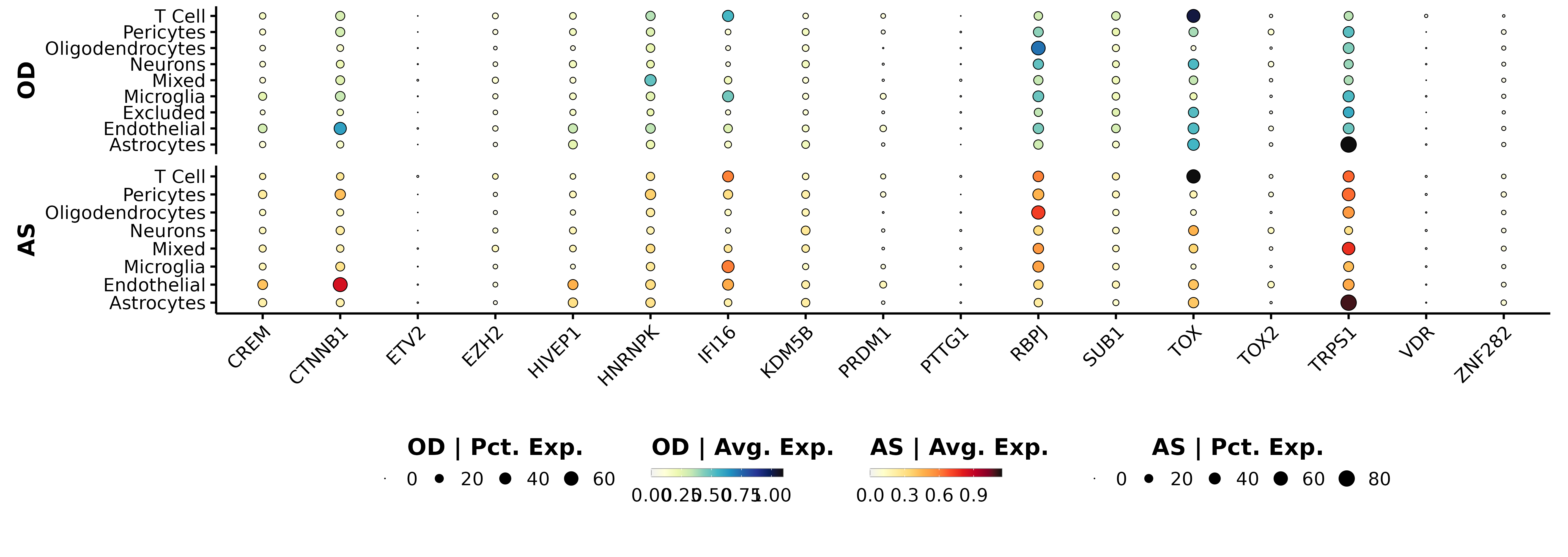
# Manually picked features from the NMF metaprograms.
features <- c("TOX", "IFI16", "RBPJ", "HNRNPK", "TRPS1",
              "CREM", "CTNNB1", "ETV2", "EZH2", "HIVEP1",
              "KDM5B", "PRDM1", "PTTG1", "SUB1", "TOX2",
              "VDR", "ZNF282") %>% sort()

sample.oligo$relabelling <- factor(sample.oligo$relabelling)
sample.astro$relabelling <- factor(sample.astro$relabelling)

p1 <- SCpubr::do_DotPlot(sample.oligo,
                         features = features,
                         group.by = "relabelling",
                         assay = "SCT",
                         legend.title = "OD | Avg. Exp.",
                         legend.length = 8,
                         legend.width = 0.5,
                         legend.framecolor = "grey50",
                         legend.tickcolor = "white",
                         legend.framewidth = 0.2,
                         legend.tickwidth = 0.2,
                         font.size = 20,
                         axis.text.face = "plain",
                         dot.scale = ) + 
      ggplot2::ylab("OD") + 
      ggplot2::theme(axis.text.x.bottom = ggplot2::element_blank(),
                     axis.ticks.x.bottom = ggplot2::element_blank(),
                     axis.line.x.bottom = ggplot2::element_blank(),
                     strip.background = ggplot2::element_blank(),
                     plot.margin = ggplot2::margin(t = 0, r = 10, b = 5, l = 10))

p2 <- SCpubr::do_DotPlot(sample.astro,
                         features = features,
                         group.by = "relabelling",
                         assay = "SCT",
                         sequential.palette = "YlOrRd",
                         legend.title = "AS | Avg. Exp.",
                         legend.length = 8,
                         legend.width = 0.5,
                         legend.framecolor = "grey50",
                         legend.tickcolor = "white",
                         legend.framewidth = 0.2,
                         legend.tickwidth = 0.2,
                         font.size = 20,
                         axis.text.face = "plain") + 
      ggplot2::ylab("AS") + 
      ggplot2::theme(strip.background = ggplot2::element_blank(),
                     strip.text = ggplot2::element_blank(),
                     plot.margin = ggplot2::margin(t = 0, r = 10, b = 0, l = 10))

p1$guides$size$title <- "OD | Pct. Exp."
p2$guides$size$title <- "AS | Pct. Exp."

p <- patchwork::wrap_plots(A = p1,
                           B = p2,
                           C = patchwork::guide_area(),
                           design = "A
                                     B
                                     C",
                           guides = "collect") + 
     patchwork::plot_annotation(theme = ggplot2::theme(legend.position = "bottom"))