Figure S6C

Code

# Enrique Blanco Carmona
# e.blancocarmona@kitz-heidelberg.de
# PhD Student – Clinical Bioinformatics
# Division of Pediatric Neurooncology (B062)
# DKFZ-KiTZ | Germany

library(Azimuth)
library(Seurat)
source("/omics/odcf/analysis/OE0145_projects/idh_gliomas/Figures_Science/revision/IDH_gliomas_book/datasets/modified_azimuth.R")
azimuth_core <- readRDS("/omics/odcf/analysis/OE0145_projects/idh_gliomas/Figures_Science/revision/IDH_gliomas_book/datasets/azimuth_core_GBmap.rds")

sample <- readRDS("/omics/odcf/analysis/OE0145_projects/idh_gliomas/Figures_Science/revision/IDH_gliomas_book/datasets/integrated_primary_OD.rds")
sample <- sample[, sample$relabelling %in% c("OPC-like", "Astro-like", "RA", "Gradient", "Cycling")]
sample$relabelling <- factor(sample$relabelling, levels = c("Astro-like", "Cycling", "Gradient", "OPC-like", "RA"))
Seurat::Idents(sample) <- sample$relabelling

Seurat::DefaultAssay(sample) <- "RNA"
sample <- Seurat::NormalizeData(sample)
sample <- Seurat::FindVariableFeatures(sample)
sample <- Seurat::ScaleData(sample)

cluster_cols <- c("RA" = "#ECA809",
                  "OPC-like" = "#043362",
                  "T Cell" = "#009FF5",
                  "Oligodendrocytes" = "#BC5210",
                  "Astrocytes" = "#279185",
                  "Microglia" = "#7EB356",
                  "Pericytes" = "#AC70FF",
                  "Mixed" = "#8d5d3f",
                  "Gradient" = "#D6D6D6",
                  "Neurons" = "#544B81",
                  "Endothelial" = "#da627d",
                  "Astro-like" = "#9A031E",
                  "Excluded" = "#4D6880",
                  "Cycling" = "#5F0F40")

sample <- Azimuth::RunAzimuth(sample, 
                              reference = azimuth_core,
                              annotation.levels = c("annotation_level_3"))


# Prepare sample metadata and apply desired cutoffs.
sample@meta.data <- sample@meta.data %>%
                    tibble::rownames_to_column(var = "cell") %>%
                    dplyr::left_join(by = "cell",
                                     y = {sample@meta.data %>%
                                          tibble::rownames_to_column(var = "cell") %>%
                                          dplyr::select(dplyr::all_of(c("cell", "predicted.annotation_level_3", "predicted.annotation_level_3.score", "mapping.score"))) %>%
                                          dplyr::rowwise() %>%
                                          dplyr::mutate("inferred_annotation" = if (.data[["predicted.annotation_level_3.score"]] >= 0.75 &
                                                                                    .data[["mapping.score"]] >= 0){.data[["predicted.annotation_level_3"]]} else {NA}) %>%
                                          dplyr::select(c("cell", "inferred_annotation"))}) %>%
                    tibble::column_to_rownames(var = "cell")

Code

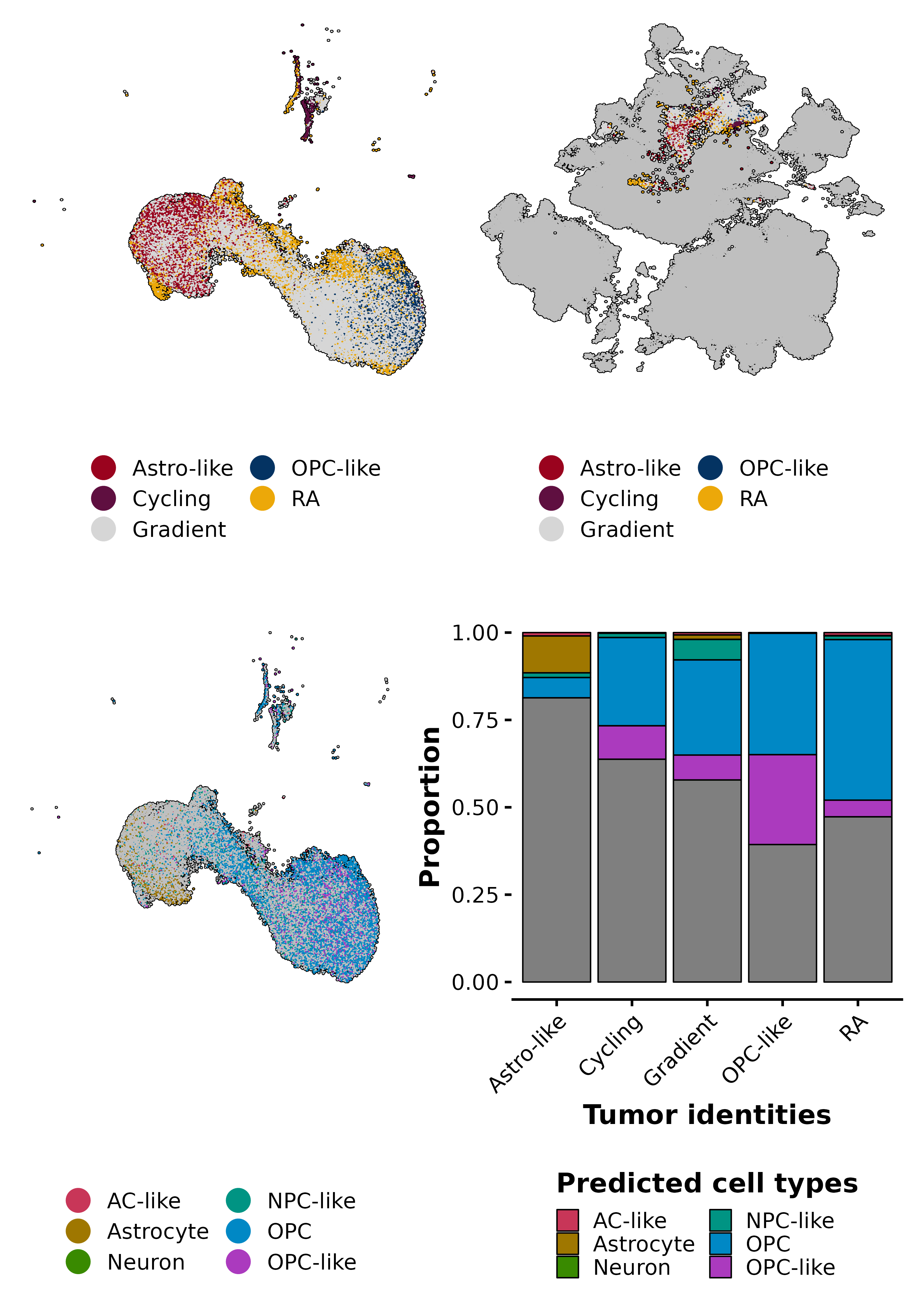
p1 <- SCpubr::do_DimPlot(sample = sample,
                         reduction = "umap",
                         colors.use = cluster_cols,
                         raster = TRUE,
                         raster.dpi = 2048,
                         pt.size = 4,
                         legend.icon.size = 8,
                         legend.ncol = 2,
                         font.size = 20)

p2 <- SCpubr::do_DimPlot(sample = sample,
                         reduction = "ref.umap",
                         colors.use = cluster_cols,
                         raster = TRUE,
                         raster.dpi = 2048,
                         pt.size = 4,
                         legend.icon.size = 8,
                         legend.ncol = 2,
                         font.size = 20)

# Add reference coordinates.
data <- as.data.frame(azimuth_core@reductions$umap@cell.embeddings)
colnames(data) <- c("x", "y")

base_layer <- scattermore::geom_scattermore(data = data,
                                            mapping = ggplot2::aes(x = .data$x,
                                                                   y = .data$y),
                                            color = "grey75",
                                            size = 4,
                                            stroke = 4 / 2,
                                            show.legend = FALSE,
                                            pointsize = 4,
                                            pixels = c(2048, 2048))
p2$layers <- append(base_layer, p2$layers)

base_layer <- scattermore::geom_scattermore(data = data,
                                            mapping = ggplot2::aes(x = .data$x,
                                                                   y = .data$y),
                                            color = "black",
                                            size = 4 * 2,
                                            stroke = 4 / 2,
                                            show.legend = FALSE,
                                            pointsize = 4 * 2,
                                            pixels = c(2048, 2048))
p2$layers <- append(base_layer, p2$layers)

p3 <- SCpubr::do_DimPlot(sample = sample,
                         reduction = "umap",
                         group.by = "inferred_annotation",
                         raster = TRUE,
                         raster.dpi = 2048,
                         pt.size = 4,
                         legend.icon.size = 8,
                         legend.ncol = 2,
                         font.size = 20)

p4 <- SCpubr::do_BarPlot(sample = sample,
                         group.by = "inferred_annotation",
                         split.by = "relabelling",
                         position = "fill",
                         legend.title = "Predicted cell types",
                         font.size = 20,
                         axis.text.face = "plain",
                         legend.ncol = 2) + 
      ggplot2::xlab("Tumor identities")

p <- (p1 | p2) / (p3 | p4)