Figure S2C

Code

# Enrique Blanco Carmona
# e.blancocarmona@kitz-heidelberg.de
# PhD Student – Clinical Bioinformatics
# Division of Pediatric Neurooncology (B062)
# DKFZ-KiTZ | Germany

cluster_cols <- c("RE" = "#ECA809",
                  "OPC-like" = "#043362",                    
                  "Gradient" = "#D6D6D6",                    
                  "Astro-like" = "#9A031E",                  
                  "Cycling" = "#5F0F40")

markers <- readRDS("/omics/odcf/analysis/OE0145_projects/idh_gliomas/Figures_Science/revision/IDH_gliomas_book/datasets/IDH_gliomas_TB_annotation_kit_with_Suva_programs_and_metaprogram_iterations.rds")
markers <- markers[c("OD_RA", "N_RA", "N2_RA")]
names(markers) <- c("OD_RE", "N_RE", "N2_RE")

sample <- readRDS("/omics/odcf/analysis/OE0145_projects/idh_gliomas/Figures_Science/revision/IDH_gliomas_book/datasets/integrated_primary_AS.rds")
sample <- sample[, sample$relabelling %in% c("OPC-like", "Astro-like", "Gradient", "RA", "Cycling")]
sample$relabelling[sample$relabelling == "RA"] <- "RE"
Seurat::Idents(sample) <- sample$relabelling

sample <- SCpubr:::compute_enrichment_scores(sample = sample,
                                             input_gene_list = markers)

list.selected <- readRDS("/omics/odcf/analysis/OE0145_projects/idh_gliomas/Figures_Science/revision/IDH_gliomas_book/datasets/RA_overlap_selected_cells_primary_AS.rds")

Code

p2 <- SCpubr::do_FeaturePlot(sample = sample, 
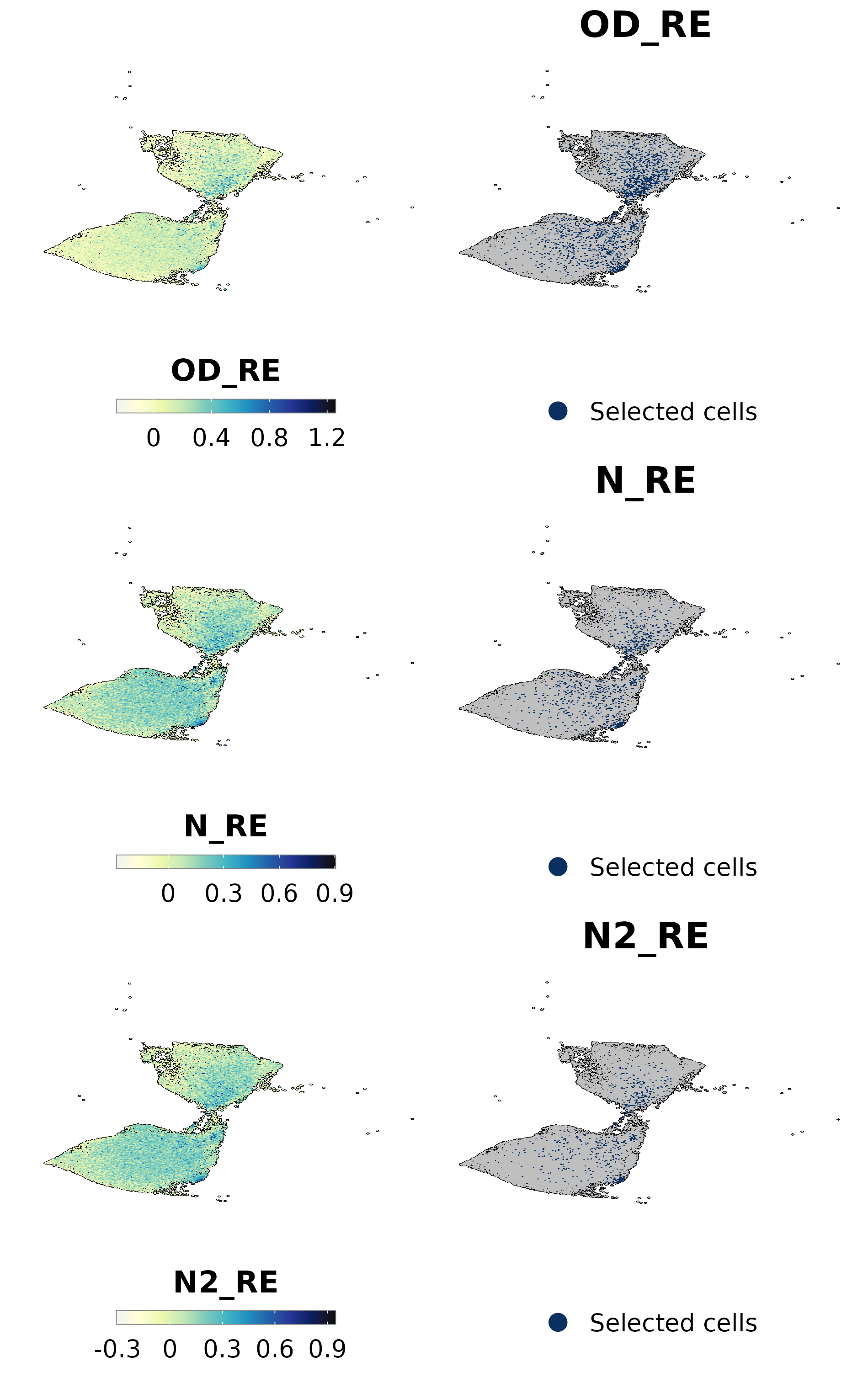
                             features = "OD_RE", 
                             font.size = 16,
                             raster = TRUE,
                             raster.dpi = 2048,
                             pt.size = 4,
                             legend.length = 8,
                             legend.width = 0.5,
                             legend.framecolor = "grey50",
                             legend.tickcolor = "white",
                             legend.framewidth = 0.2,
                             legend.tickwidth = 0.2,
                             order = TRUE) + ggplot2::theme(plot.margin = ggplot2::margin(t = 0, r = 0, b = 0, l = 0))

p3 <- SCpubr::do_FeaturePlot(sample = sample, 
                             features = "N_RE", 
                             font.size = 16,
                             raster = TRUE,
                             raster.dpi = 2048,
                             pt.size = 4,
                             legend.length = 8,
                             legend.width = 0.5,
                             legend.framecolor = "grey50",
                             legend.tickcolor = "white",
                             legend.framewidth = 0.2,
                             legend.tickwidth = 0.2,
                             order = TRUE) + ggplot2::theme(plot.margin = ggplot2::margin(t = 0, r = 0, b = 0, l = 0))

p4 <- SCpubr::do_FeaturePlot(sample = sample, 
                             features = "N2_RE", 
                             font.size = 16,
                             raster = TRUE,
                             raster.dpi = 2048,
                             pt.size = 4,
                             legend.length = 8,
                             legend.width = 0.5,
                             legend.framecolor = "grey50",
                             legend.tickcolor = "white",
                             legend.framewidth = 0.2,
                             legend.tickwidth = 0.2,
                             order = TRUE) + ggplot2::theme(plot.margin = ggplot2::margin(t = 0, r = 0, b = 0, l = 0))

p5 <- SCpubr::do_DimPlot(sample = sample, 
                         cells.highlight = list.selected$O_RA, 
                         font.size = 16,
                         raster = TRUE,
                         raster.dpi = 2048,
                         pt.size = 4,
                         plot.title = "OD_RE") + ggplot2::theme(plot.title = ggplot2::element_text(hjust = 0.5),
                                                                plot.margin = ggplot2::margin(t = 0, r = 0, b = 0, l = 0))

p6 <- SCpubr::do_DimPlot(sample = sample, 
                         cells.highlight = list.selected$N_RA, 
                         font.size = 16,
                         raster = TRUE,
                         raster.dpi = 2048,
                         pt.size = 4,
                         plot.title = "N_RE") + ggplot2::theme(plot.title = ggplot2::element_text(hjust = 0.5),
                                                               plot.margin = ggplot2::margin(t = 0, r = 0, b = 0, l = 0))

p7 <- SCpubr::do_DimPlot(sample = sample, 
                         cells.highlight = list.selected$N2_RA, 
                         font.size = 16,
                         raster = TRUE,
                         raster.dpi = 2048,
                         pt.size = 4,
                         plot.title = "N2_RE") + ggplot2::theme(plot.title = ggplot2::element_text(hjust = 0.5),
                                                                plot.margin = ggplot2::margin(t = 0, r = 0, b = 0, l = 0))

p8 <- SCpubr::do_CorrelationPlot(input_gene_list = list.selected, 
                                 mode = "jaccard", 
                                 font.size = 16,
                                 axis.text.face = "plain",
                                 legend.length = 8,
                                 legend.width = 0.5,
                                 legend.framecolor = "grey50",
                                 legend.tickcolor = "white",
                                 legend.framewidth = 0.2,
                                 legend.tickwidth = 0.2) + ggplot2::theme(plot.margin = ggplot2::margin(t = 0, r = 0, b = 0, l = 0))

layout <-  "CF
            DG
            EH"
p <- patchwork::wrap_plots(C = p2,
                           D = p3,
                           E = p4,
                           F = p5,
                           G = p6,
                           H = p7,
                           design = layout)