Figure S3G

Code

# Inma Hernandez Lopez
# inmaculada.hernandez-lopez@ukr.de
# LIT -  Leibniz-Institute für Immunotherapie

# Marc Elosua Bayés
# marc.elosua@cnag.crg.eu
# CNAG - CRG

# Enrique Blanco Carmona
# e.blancocarmona@kitz-heidelberg.de
# PhD Student – Clinical Bioinformatics
# Division of Pediatric Neurooncology (B062)
# DKFZ-KiTZ | Germany

proportions <- readRDS("/omics/odcf/analysis/OE0145_projects/idh_gliomas/Figures_Science/revision/IDH_gliomas_book/datasets/spotlight_deconv_olig_CGGA.rds")
proportions <- proportions$mat %>% 
               data.frame(check.names = FALSE) %>%
               tibble::rownames_to_column("ID") %>%
               tidyr::pivot_longer(cols = -ID,
                                   names_to = "cell_type",
                                   values_to = "proportion")
proportions$cell_type[proportions$cell_type == "RA"] <- "RE"

proportions <- proportions %>% 
               dplyr::mutate("ID" = factor(.data$ID, levels = {proportions %>% dplyr::filter(.data$cell_type == "RE") %>% dplyr::arrange(dplyr::desc(.data$proportion)) %>% dplyr::pull("ID")}))

cluster_cols <- c("RE" = "#ECA809",
                  "OPC-like" = "#043362",                    
                  "T Cell" = "#009FF5",                   
                  "Oligodendrocytes" = "#BC5210",            
                  "Astrocytes" = "#279185",                  
                  "Microglia" = "#7EB356",                   
                  "Pericytes" = "#AC70FF",                  
                  "Mixed" = "#8d5d3f",                   
                  "Gradient" = "#D6D6D6",                    
                  "Neurons" = "#544B81",                   
                  "Endothelial" = "#da627d",                 
                  "Astro-like" = "#9A031E",               
                  "Cycling" = "#5F0F40")

Code

p0 <- proportions %>% 
      ggplot2::ggplot(mapping = ggplot2::aes(x = .data$ID,
                                             y = .data$proportion,
                                             fill = .data$cell_type)) + 
      ggplot2::geom_col(color = "black", position = "fill", linewidth = 0.25) + 
      ggplot2::scale_fill_manual(values = cluster_cols, name = "") + 
      ggplot2::theme_minimal(base_size = 20) +
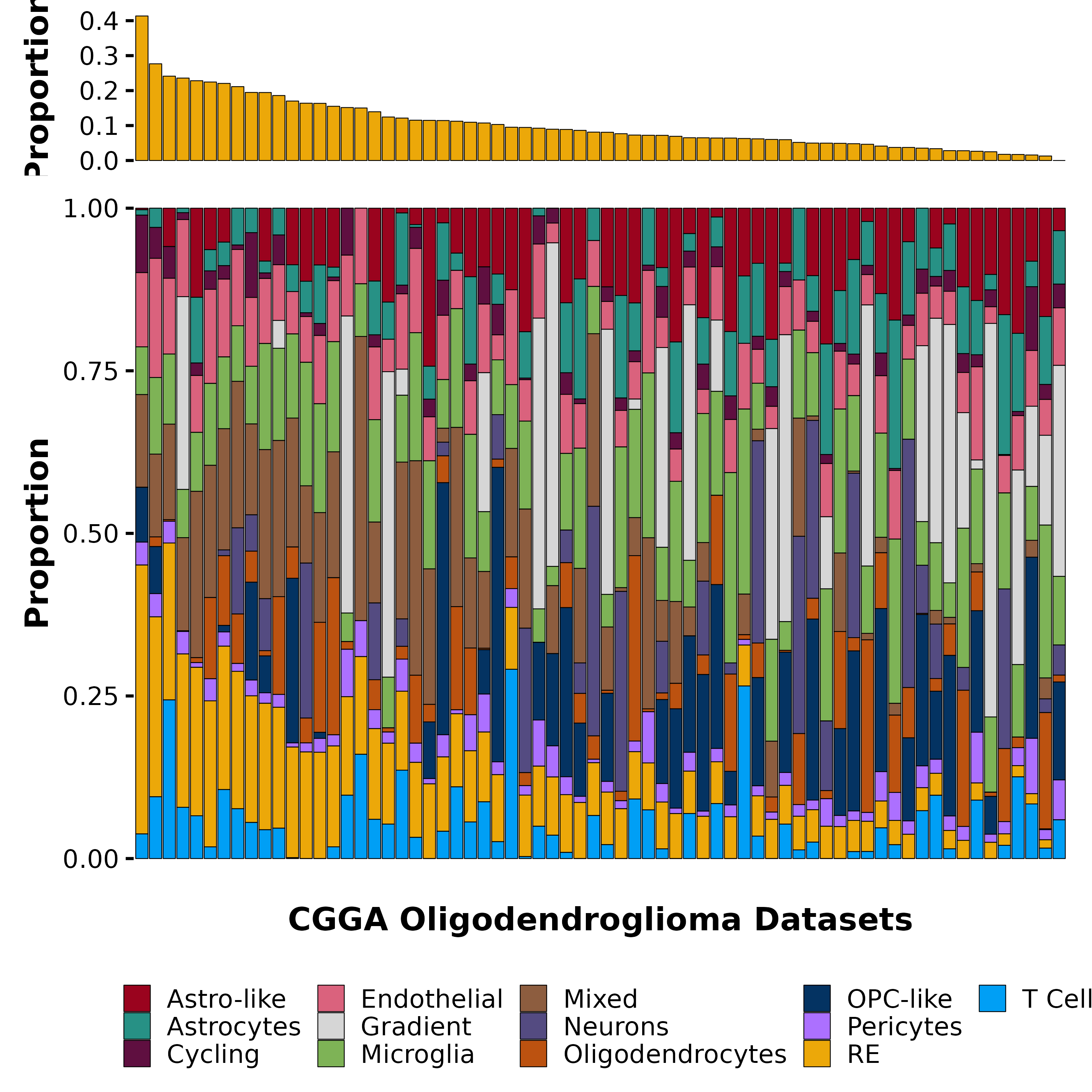
      ggplot2::labs(x = "CGGA Oligodendroglioma Datasets",
                    y = "Proportion") +
      ggplot2::theme(axis.title = ggplot2::element_text(color = "black",
                                                        face = "bold"),
                     axis.line.x = ggplot2::element_blank(),
                     axis.line.y = ggplot2::element_blank(),
                     axis.text.x = ggplot2::element_blank(),
                     axis.text.y = ggplot2::element_text(color = "black", face = "plain"),
                     axis.ticks.y = ggplot2::element_line(color = "black"),
                     axis.ticks.x = ggplot2::element_blank(),
                     plot.title.position = "plot",
                     plot.title = ggplot2::element_text(face = "bold", hjust = 0.5),
                     plot.subtitle = ggplot2::element_text(face = "plain", hjust = 0),
                     plot.caption = ggplot2::element_text(face = "plain", hjust = 1),
                     panel.grid = ggplot2::element_blank(),
                     text = ggplot2::element_text(family = "sans"),
                     plot.caption.position = "plot",
                     legend.text = ggplot2::element_text(face = "plain"),
                     legend.position = "bottom",
                     legend.title = ggplot2::element_text(face = "bold"),
                     legend.justification = "center",
                     plot.margin = ggplot2::margin(t = 0, r = 10, b = 0, l = 10),
                     plot.background = ggplot2::element_rect(fill = "white", color = "white"),
                     panel.background = ggplot2::element_rect(fill = "white", color = "white"),
                     legend.background = ggplot2::element_rect(fill = "white", color = "white"),
                     strip.text = ggplot2::element_text(color = "black", face = "bold"),
                     strip.background = ggplot2::element_blank())

p1 <- proportions %>% 
      dplyr::filter(.data$cell_type == "RE") %>% 
      ggplot2::ggplot(mapping = ggplot2::aes(x = .data$ID,
                                             y = .data$proportion,
                                             fill = .data$cell_type)) + 
      ggplot2::geom_col(color = "black", position = "stack", linewidth = 0.25) + 
      ggplot2::scale_fill_manual(values = cluster_cols, name = "") + 
      ggplot2::theme_minimal(base_size = 20) +
      ggplot2::labs(x = "",
                    y = "Proportion") +
      ggplot2::theme(axis.title.y = ggplot2::element_text(color = "black",
                                                          face = "bold"),
                     axis.title.x = ggplot2::element_blank(),
                     axis.line.x = ggplot2::element_blank(),
                     axis.line.y = ggplot2::element_blank(),
                     axis.text.x = ggplot2::element_blank(),
                     axis.text.y = ggplot2::element_text(color = "black", face = "plain"),
                     axis.ticks.y = ggplot2::element_line(color = "black"),
                     axis.ticks.x = ggplot2::element_blank(),
                     plot.title.position = "plot",
                     plot.title = ggplot2::element_blank(),
                     plot.subtitle = ggplot2::element_text(face = "plain", hjust = 0),
                     plot.caption = ggplot2::element_text(face = "plain", hjust = 1),
                     panel.grid = ggplot2::element_blank(),
                     text = ggplot2::element_text(family = "sans"),
                     plot.caption.position = "plot",
                     legend.text = ggplot2::element_text(face = "plain"),
                     legend.position = "none",
                     legend.title = ggplot2::element_text(face = "bold"),
                     legend.justification = "center",
                     plot.margin = ggplot2::margin(t = 0, r = 10, b = 0, l = 10),
                     plot.background = ggplot2::element_rect(fill = "white", color = "white"),
                     panel.background = ggplot2::element_rect(fill = "white", color = "white"),
                     legend.background = ggplot2::element_rect(fill = "white", color = "white"),
                     strip.text = ggplot2::element_text(color = "black", face = "bold"),
                     strip.background = ggplot2::element_blank())

p <- patchwork::wrap_plots(list(p1, p0), ncol = 1, heights = c(0.2, 0.9))